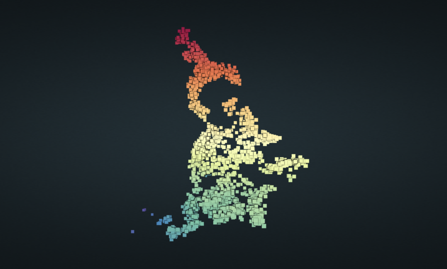
3D RECONSTRUCTION WITH OPENCV AND OPEN3D

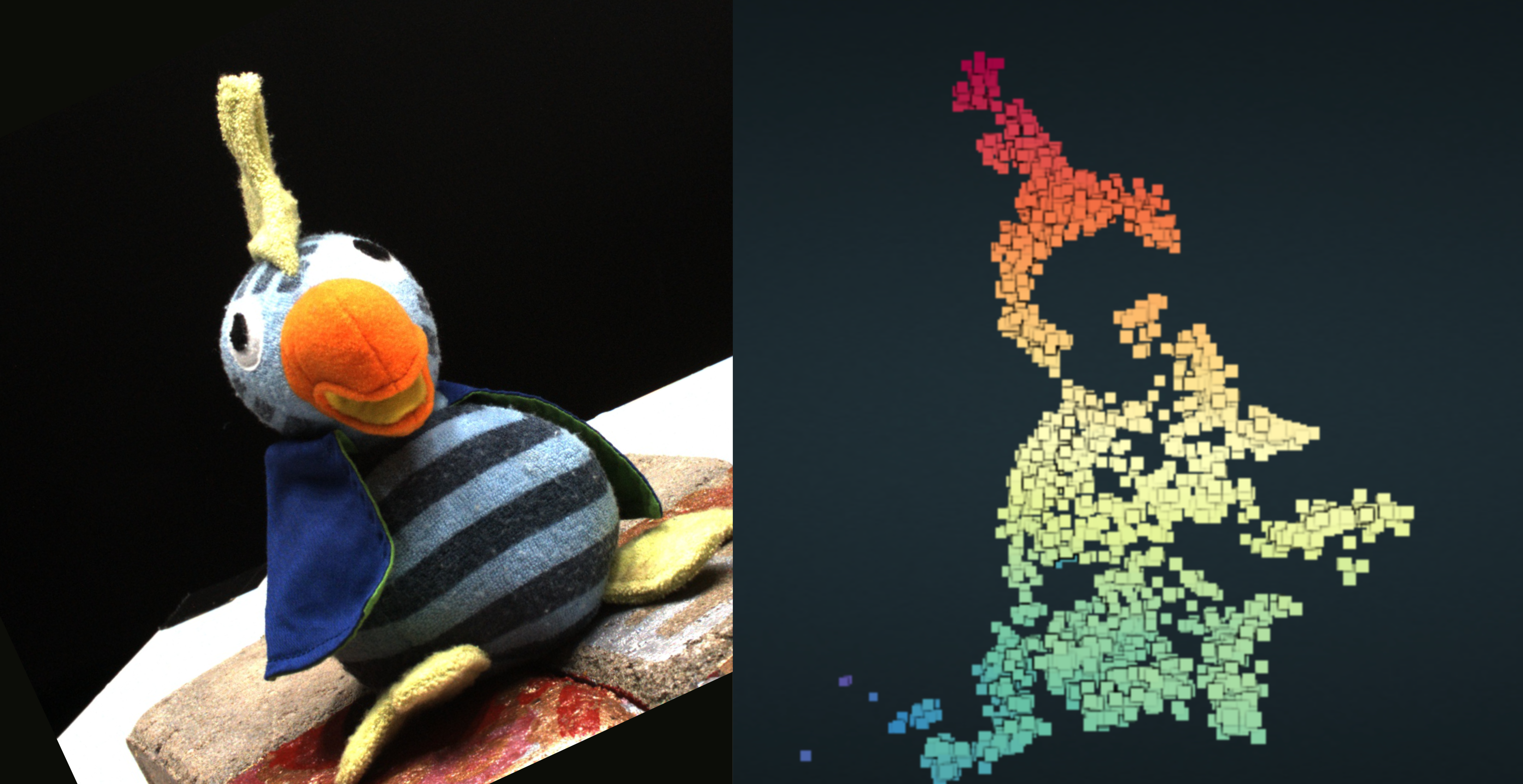
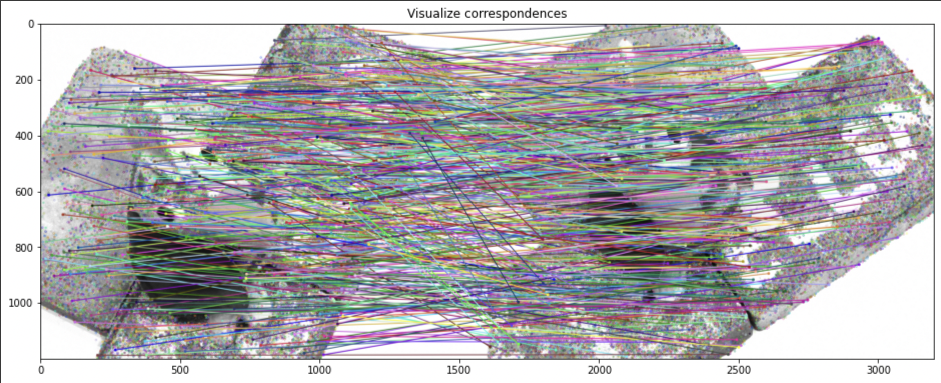
There is no denying that 3D reconstruction is an incredibly useful and powerful tool to have as a computer scientist. It is helpful in fields such as medicine and virtual reality because it allows for a complete interactive rendering of a person or object that can be accessed at any time and at any angle. In my approach to implement 3D reconstruction, I started from the beginning. Much like I did the Shi-Tomasi corner detection before, in this implementation I used SIFT, an even more powerful detection algorithm. I used the tutorial on opencv.org to get the keypoints and descriptors of each image. This step is important because it allows me to spot the points of interest. Next is time to start the reconstruction. I first used two images and found their correspondences using SIFT and the BFMatcher function’s knnMatch to find the matching points. But this didn’t give me that great of accuracy and gave me above 2000 corresponding points (Most looked incorrect), so I had to perform a ratio test. In this ratio test, I was checking if the distances between match distances was less than a certain value. I found that 0.88 was a good number to multiply against the second value of the current match and gave me less points that produced more accurate results.

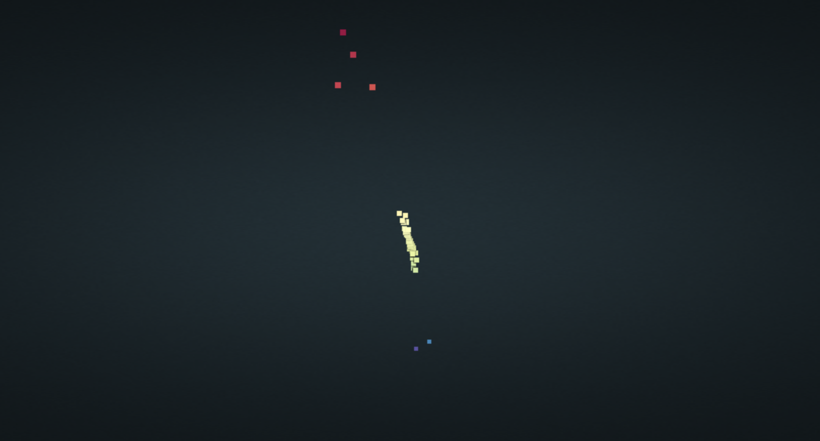
Next, I reconstructed the 3D points with triangulation using the OpenCV function triangulatePoints(), and in order to find the Camera matrix, I used the same method I implemented in a different project to do so. This was simply finding the dot product of the intrinsic matrix to the extrinsic matrix. When I visualized this, all I saw was a line of points on the screen, which was concerning, but I kept moving forward because I thought my further optimizations will fix this.

Now it was time to include the other 46 images. But before that, I needed to make sure that my correspondence was noise free and remove false correspondences. This part was very challenging for me, I was having trouble trying to extract the R and t matrices from the extrinsic matrices. After lots of research, I was able to determine that a simple multiplication between the second extrinsic matrix and the inverse of the first extrinsic matrix would produce my essential matrix. From there, I would know that the 4th column was my t, and the 3x3 matrix to the left of that (columns 1-3) is my R. With this, I converted my t to t_cross, and used the same way I created the fundamental matrix in a different project with my new t_cross * R matrix. With my fundamental matrix, it would be time to remove outliers. This part was challenging as well, but after looking back at a different project’s RANSAC algorithm that I implemented, I was able to use parts of that algorithm to find the inlier x, y coordinates from point 1 and point 2 and return them. I had to fine tune the threshold in this and found 10 to be a good number. This reduced my number of correspondences to be more accurate. I ran the code that added more cameras, which took more than 6 minutes to complete. I visualized the results, only to find it was difficult to see anything that looks close to our photographed object.

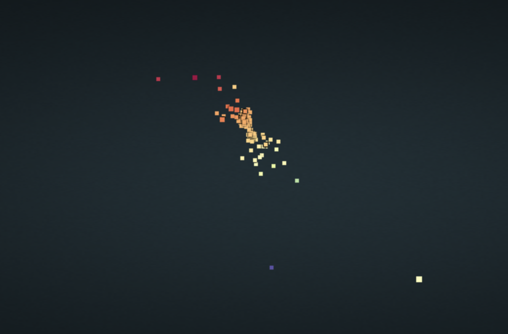
Time for optimizations! First, I needed to install the powerful package Open3D. Open3D would allow me to manipulate the point cloud and remove those pesky outliers. Because the Open3D visualizer doesn’t work with colab, I needed to use the pypotree visualizer. I first converted the numpy array to an Open3D pointcloud, allowing me to use Open3D methods. Then, I downsampled the point cloud using the voxel_size 0.001, I had first tried 0.02, but I found 0.001 produced a better result. Then it was time to remove outliers. There are two functions I tried, first was the statistical outlier removal, which no matter what settings I put, I couldn’t produce the correct construction. The second was the radius outlier removal, and after some tweaking of the parameters which made the radius of what would be considered inliers or outliers, I finally was able to produce a correct 3D pointcloud. I then converted from a Open3D pointcloud back to a numpy array, and visualized it using pypotree.